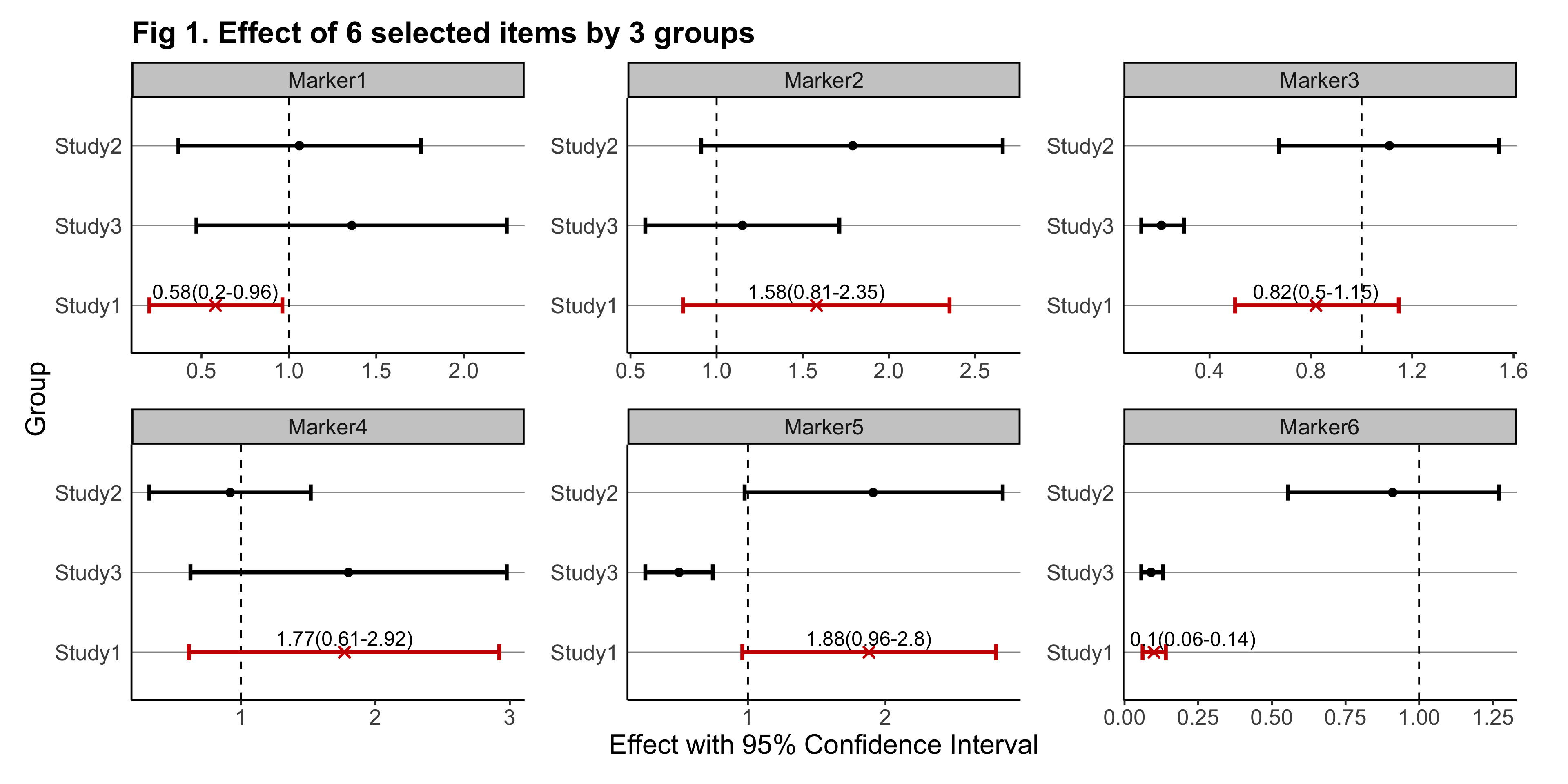
The goal of gwasforest is to extract and reform data from GWAS results, and then make a single integrated forest plot containing multiple windows of which each shows the result of individual SNPs (or other items of interest).
Installation
The official release version of gwasforest can be installed from CRAN with:
utils::install.packages("gwasforest")The development version of gwasforest can be installed from GitHub with:
devtools::install_github("yilixu/gwasforest", ref = "main")Quick Demos
- ( 1 ) when customFilename (main input) is in dataframe format (with standardized column names):
library(gwasforest)
set.seed(123)

# generate example data
tempValue = runif(n = 18, min = 0.01, max = 2)
tempStdErr = tempValue / rep(3:5, times = 6)
eg_customFilename = data.frame(paste0("Marker", 1:6), tempValue[1:6], tempStdErr[1:6], tempValue[7:12], tempStdErr[7:12], tempValue[13:18], tempStdErr[13:18], stringsAsFactors = FALSE)
colnames(eg_customFilename) = c("MarkerName", paste0(rep("Study", times = 6), rep(1:3, each = 2), rep(c("__Value", "__StdErr"), times = 3)))
rm(tempValue, tempStdErr)

# take a quick look at the example: main input data (with standardized column names)
print(eg_customFilename)
#>   MarkerName Study1__Value Study1__StdErr Study2__Value Study2__StdErr
#> 1    Marker1     0.5822793     0.19409309     1.0609299      0.3536433
#> 2    Marker2     1.5787272     0.39468180     1.7859139      0.4464785
#> 3    Marker3     0.8238641     0.16477281     1.1073557      0.2214711
#> 4    Marker4     1.7672046     0.58906821     0.9186633      0.3062211
#> 5    Marker5     1.8815299     0.47038247     1.9140984      0.4785246
#> 6    Marker6     0.1006574     0.02013149     0.9121350      0.1824270
#>   Study3__Value Study3__StdErr
#> 1    1.35836556     0.45278852
#> 2    1.14954047     0.28738512
#> 3    0.21482012     0.04296402
#> 4    1.80065169     0.60021723
#> 5    0.49971459     0.12492865
#> 6    0.09369847     0.01873969
# run gwasforest function
eg_returnList = gwasforest(eg_customFilename, stdColnames = TRUE, valueFormat = "Effect", metaStudy = "Study1", colorMode = "duo")
#> [1] "Column names are in the same format as instruction example"
#> [1] "Loading user-provided values"
#> [1] "Start calculating Confidence Interval (non-exponential)"
#> [1] "Based on user's choice, GWAS results output file will not be generated"
#> [1] "All studies except meta study will be set in alphabetical order from top to bottom on the forest plot"
#> Registered S3 methods overwritten by 'ggplot2':
#>   method         from
#>   [.quosures     rlang
#>   c.quosures     rlang
#>   print.quosures rlang
#> [1] "Based on user's choice, GWAS forest plot file will not be generated"
#> [1] "Run completed, thank you for using gwasforest"- ( 2 ) when customFilename is in dataframe format (without standardized column names), while customFilename_studyName is provided in dataframe format:
# generate example data
tempValue = runif(n = 18, min = 0.01, max = 2)
tempStdErr = tempValue / rep(3:5, times = 6)
eg_customFilename2 = data.frame(paste0("Marker", 1:6), tempValue[1:6], tempStdErr[1:6], tempValue[7:12], tempStdErr[7:12], tempValue[13:18], tempStdErr[13:18], stringsAsFactors = FALSE)
colnames(eg_customFilename2) = c("MarkerName", paste0(rep("Study", times = 6), rep(1:3, each = 2), sample(LETTERS, 6)))
rm(tempValue, tempStdErr)
eg_customFilename_studyName = data.frame("studyName" = paste0("Study", 1:3), stringsAsFactors = FALSE)

# take a quick look at the example: main input data (without standardized column names)
print(eg_customFilename2)
#>   MarkerName   Study1K   Study1G   Study2U    Study2L    Study3O
#> 1    Marker1 0.6625622 0.2208541 1.3148545 0.43828485 1.92641822
#> 2    Marker2 1.9094623 0.4773656 1.4199756 0.35499391 1.80557510
#> 3    Marker3 1.7801832 0.3560366 1.0926914 0.21853828 1.38450350
#> 4    Marker4 1.3886788 0.4628929 1.1923426 0.39744754 1.59298016
#> 5    Marker5 1.2846086 0.3211521 0.5854279 0.14635697 0.05898123
#> 6    Marker6 1.9885969 0.3977194 0.3027562 0.06055123 0.96081398
#>      Study3J
#> 1 0.64213941
#> 2 0.45139377
#> 3 0.27690070
#> 4 0.53099339
#> 5 0.01474531
#> 6 0.19216280

# take a quick look at the example: custom study name
print(eg_customFilename_studyName)
#>   studyName
#> 1    Study1
#> 2    Study2
#> 3    Study3
# run gwasforest function
eg_returnList2 = gwasforest(eg_customFilename2, customFilename_studyName = eg_customFilename_studyName, stdColnames = FALSE, customColnames = c("Value", "StdErr"), valueFormat = "Effect", metaStudy = "Study1", colorMode = "duo")
#> [1] "Column names are grouped by study and in the order of |Value, StdErr|"
#> [1] "Start reforming"
#> [1] "Loading user-provided values"
#> [1] "Start calculating Confidence Interval (non-exponential)"
#> [1] "Based on user's choice, GWAS results output file will not be generated"
#> [1] "As per user's request, all studies except meta study will be set in the original order from top to bottom on the forest plot"
#> [1] "Based on user's choice, GWAS forest plot file will not be generated"
#> [1] "Run completed, thank you for using gwasforest"- ( 3 ) when customFilename_results is in dataframe format (run either of the two steps above to see the example results):
# extract results table
eg_customFilename_results = eg_returnList[[1]]

# take a quick look at the example: results table
print(eg_customFilename_results)
#>    MarkerName Value     Upper      Lower StudyName              CI
#> 1     Marker1  0.58 0.9627017 0.20185681    Study1  0.58(0.2-0.96)
#> 2     Marker2  1.58 2.3523036 0.80515088    Study1 1.58(0.81-2.35)
#> 3     Marker3  0.82 1.1468188 0.50090936    Study1  0.82(0.5-1.15)
#> 4     Marker4  1.77 2.9217783 0.61263094    Study1 1.77(0.61-2.92)
#> 5     Marker5  1.88 2.8034795 0.95958025    Study1  1.88(0.96-2.8)
#> 6     Marker6  0.10 0.1401151 0.06119972    Study1  0.1(0.06-0.14)
#> 7     Marker1  1.06 1.7540708 0.36778904    Study2 1.06(0.37-1.75)
#> 8     Marker2  1.79 2.6610117 0.91081609    Study2 1.79(0.91-2.66)
#> 9     Marker3  1.11 1.5414391 0.67327225    Study2 1.11(0.67-1.54)
#> 10    Marker4  0.92 1.5188567 0.31846995    Study2 0.92(0.32-1.52)
#> 11    Marker5  1.91 2.8520066 0.97619016    Study2 1.91(0.98-2.85)
#> 12    Marker6  0.91 1.2696919 0.55457806    Study2 0.91(0.55-1.27)
#> 13    Marker1  1.36 2.2458311 0.47090006    Study3 1.36(0.47-2.25)
#> 14    Marker2  1.15 1.7128153 0.58626564    Study3 1.15(0.59-1.71)
#> 15    Marker3  0.21 0.2990296 0.13061063    Study3  0.21(0.13-0.3)
#> 16    Marker4  1.80 2.9770775 0.62422592    Study3  1.8(0.62-2.98)
#> 17    Marker5  0.50 0.7445747 0.25485444    Study3  0.5(0.25-0.74)
#> 18    Marker6  0.09 0.1304283 0.05696867    Study3 0.09(0.06-0.13)
library(ggplot2)

# render plot, see additional NOTES below
plot(eg_returnList[[2]])
#> Warning: Removed 12 rows containing missing values (geom_text_repel).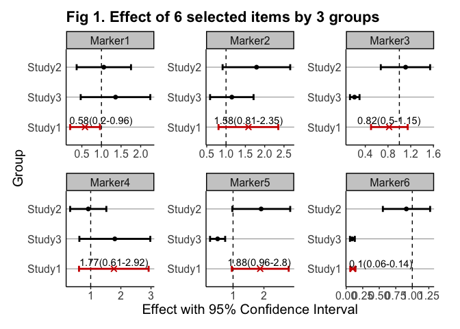
- ( 4 ) NOTES: As shown above, the plot rendered through plot() may suffer from certain issues such as low-resolution and overlapping labels. To overcome these issues and get the genuine plot output from gwasforest, it is recommended to provide a valid outputFolderPath so that a better-rendered plot can be created. The below is the genuine plot output created from the same example data: